Solvers
General information
The goal is to compute the voltages at each bus and the currents and powers flow in each branch of the network. The computation must respect Kirchhoff’s laws and the constraints of the network.
More formally, this is done by solving a system of \(n\) nonlinear equations with \(n\) variables:
The goal is then to find \(x\) such that:
Computationally, this translates to finding a solution \(x\) such that:
With \(\varepsilon\) being a small tolerance. In code, \(\varepsilon\) can be set with en.solve_load_flow(tolerance=...)
(by default 1e-6).
There are several solvers to solve this kind of problems. In Roseau Load Flow, the following solvers are available:
Newton-Raphson
This is the classical Newton-Raphson method.
First, an initial solution \(x_0\) is chosen by initializing the voltages either by propagating the voltage of the sources
or by re-using the results from the last successful run. The choice of either option depends on the warm_start
argument to the en.solve_load_flow() method.
Then, multiple iterations are made with:
with \(J_F\) being the jacobian of \(F\).
The algorithm stops when it finds a solution \(x_k\) such that \(||F(x_k)||_{\infty} < \varepsilon\) within a maximum number
of iterations (modify with en.solve_load_flow(max_iterations=...)). If the maximum number of iterations is exceeded,
the solver did not converge and the execution fails.
Parameters
The Newton-Raphson solver doesn’t accept any parameter.
Goldstein and Price
This is a variant of the classical Newton-Raphson solver with a linear search.
At each iteration, \(x_{k+1}\) is calculated using:
with \(d = -J_F^{-1}F\)
For the classical Newton-Raphson solver, \(t=1\) is chosen for the next iterate. The idea of the linear searches, in this case the Goldstein and Price variant, is to find a “better” \(t\) that improves the convergence of the solver.
Let \(g\) be a function to be minimized:
Let \(q\) be the function \(g\) in the direction \(d\):
A search is made to find \(t\) such that:
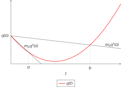
In the figure above, any \(t\) such that \(a < t < b\) is satisfactory.
This \(t\) is found by dichotomy with multiple iterations, but in most cases only one iteration is needed. This is especially true when there are no flexible loads in the network.
\(t\) is then used to compute \(x_{k+1} = x_k + t d(x_k)\)
The Goldstein and Price variant is thus as fast as the classical Newton-Raphson while being more robust.
Parameters
The Goldstein and Price solver accepts the following parameters:
"m1"the first constant of the Goldstein and Price variant. By default:0.1."m2"the second constant of the Goldstein and Price variant. By default:0.9. Note that the constraint \(m_1 < m_2\) must be met."weighted_merit"whether to scale the residuals before applying the search criterion above. By default:True. See below.
Weighted merit function
The criterion (3) compares residuals against each other, but the entries of \(F\) are not all on the same scale. How large a residual gets for a given error depends on the equation it comes from: a bus fed through a very low impedance produces a current mismatch orders of magnitude above one at the end of a long, weakly connected feeder, and a load under a steep voltage-dependent control law produces a larger one still. Measured by the raw norm \(||F||_2\), the small-scale equations are nearly invisible: the line search can accept a step that quietly wrecks one of them as long as the large-scale equations improve.
When weighted_merit is enabled (default), each residual is divided by \(\max(1, ||J_i||_\infty)\), the infinity norm of
its own Jacobian row, before the norm is taken:
The weights are recomputed from the current Jacobian at every iteration. This changes only which candidate \(t\) is
accepted; the convergence check against tolerance and the residual returned by solve_load_flow both stay on the raw,
physical residuals.
Backward-Forward
This is an implementation of the backward-forward sweep method, which offers an efficient alternative to traditional Newton-Raphson algorithms.
Advantages
Faster Execution Time: The backward-forward sweep method generally executes more quickly than Newton-Raphson-based approaches.
Limitations
Modeling Restrictions:
The network cannot contain loops.
Floating neutrals are not allowed for loads and sources.
Convergence: This method may exhibit weaker convergence properties, particularly in scenarios involving flexible loads.
Important Note
This solver is still in the experimental stage. Users should be aware that certain edge cases may not be handled correctly when utilizing the backward-forward sweep method. If you face any issues with this solver, please let us know by filing a GitHub issue
Parameters
The Backward-Forward solver doesn’t accept any parameter.