Plotting

Roseau Load Flow provides functions to plot networks and some electric quantities in the roseau.load_flow.plotting module.

Plotting a network on a map

The plot_interactive_map() function plots an ElectricalNetwork on an interactive map using the folium library. The function requires the geometries of the elements in the network to be defined. Only buses and lines are currently plotted. Simply call the function with an ElectricalNetwork to get an interactive map of the network plot_interactive_map(en).

The plot_interactive_map function uses the ElectricalNetwork geo dataframes of buses and lines to plot the network on a map. The function accepts optional arguments to customize the appearance of the plot. Refer to the function’s documentation for more information.

Let’s take a MV network from the catalogue as an example to show how we can customize the style of the buses on the map:

>>> import roseau.load_flow as rlf
>>> from roseau.load_flow.plotting import plot_interactive_map
>>> en = rlf.ElectricalNetwork.from_catalogue(name="MVFeeder210", load_point_name="Winter")
>>> en
<ElectricalNetwork: 128 buses, 126 lines, 0 transformers, 1 switch, 82 loads, 1 source, 1 ground, 1 potential ref>

As the id of the buses of this network contains information about the type of bus, we can use it to apply different styles for different bus types. For example, HV/MV substation can have different size and color than MV/LV substations and junction buses. plot_interactive_map takes an optional style_function argument to customize the style of the plots. This is a function that accepts a GeoJSON feature mapping and returns an optional dictionary of style properties. The GeoJSON feature contains an "element_type" property that indicates the type of the element (bus, line, etc.). The other properties are the columns of the dataframes of the elements of the network.

>>> def style_function(feature: dict) -> dict | None:
...     # If the element is not a bus, return None to use the default style
...     if feature["properties"]["element_type"] != "bus":
...         return None
...     # Override the default style of buses based on the bus id
...     bus_id = feature["properties"]["id"]
...     if bus_id.startswith("HVMV"):  # HV/MV substation
...         return {
...             "fill": True,
...             "fillColor": "#000000",
...             "color": "#000000",
...             "fillOpacity": 1,
...             "radius": 7,
...         }
...     elif bus_id.startswith("MVLV"):  # MV/LV substations
...         return {
...             "fill": True,
...             "fillColor": "#234e83",
...             "color": "#234e83",
...             "fillOpacity": 1,
...             "radius": 5,
...         }
...     else:  # Junction buses
...         return {
...             "fill": True,
...             "fillColor": "#234e83",
...             "color": "#234e83",
...             "fillOpacity": 1,
...             "radius": 3,
...         }
...

Finally, calling the plot_interactive_map function with the custom style function produces an interactive map of the network:

>>> m = plot_interactive_map(en, style_function=style_function)
>>> m

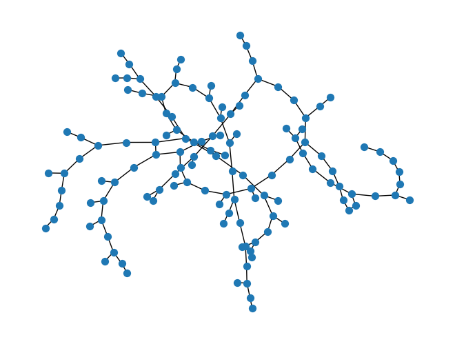
Plotting a network with no geometries

If the network does not have geometries defined for its elements, the plot_interactive_map function will not work. In this case, you can use the to_graph() method to convert the network to a networkx Graph and plot it using the networkx library. In the following example we plot the graph of the network MVFeeder210 from the previous example:

>>> import networkx as nx
... import roseau.load_flow as rlf
... en = rlf.ElectricalNetwork.from_catalogue(name="MVFeeder210", load_point_name="Winter")
... for bus in en.buses.values():
...     bus.geometry = None  # Pretend buses don't have geometries
... G = en.to_graph()
... nx.draw(G, node_size=50)  # This works even if the geometries are not defined

See the networkx docs for more information.

Plotting voltage phasors

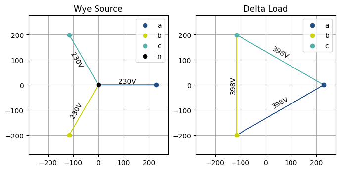
The plot_voltage_phasors() function plots the voltage phasors of a bus, load or source in the complex plane. This function can be used to visualize voltage unbalance in multi-phase systems for instance. It takes the element and an optional matplotlib Axes object to use for the plot. Note that the element must have load flow results to plot the voltage phasors.

>>> import matplotlib.pyplot as plt
... import roseau.load_flow as rlf
... from roseau.load_flow.plotting import plot_voltage_phasors

>>> bus = rlf.Bus("Bus", phases="abcn")
... source = rlf.VoltageSource("Wye Source", bus, voltages=230, phases="abcn")
... load = rlf.ImpedanceLoad("Delta Load", bus, impedances=50, phases="abc")
... rlf.PotentialRef("PRef", element=bus)
... en = rlf.ElectricalNetwork.from_element(bus)
... en.solve_load_flow()

>>> fig, axes = plt.subplots(1, 2, figsize=(8, 4))
... plot_voltage_phasors(source, ax=axes[0])
... plot_voltage_phasors(load, ax=axes[1])
... plt.show()

A similar function plot_symmetrical_voltages() plots the symmetrical components of the voltage phasors of a three-phase bus, load or source.